How To Write Vlookup Formula, Example, Syntax, Definition Of Vlookup Function

The vlookup formula is a common business tool used to refer to data in one spreadsheet and retrieve data that matches what we are looking for.

The vlookup formula is a function that searches for a specific text string in one column of data and then finds all the values in the same row or column as it.

A vlookup formula is most often used when you want to show a list of values that match a specific name or value. Learn here how to use the vlookup formula to find specific data in one column or row and show matching data in another column or row.

How to write or apply Vlookup formula In Excel

The first step of using the vlookup formula is to understand that there are multiple functions that can be used depending on the situation. One way to write a vlookup formula is by referring to a specific column and row number.

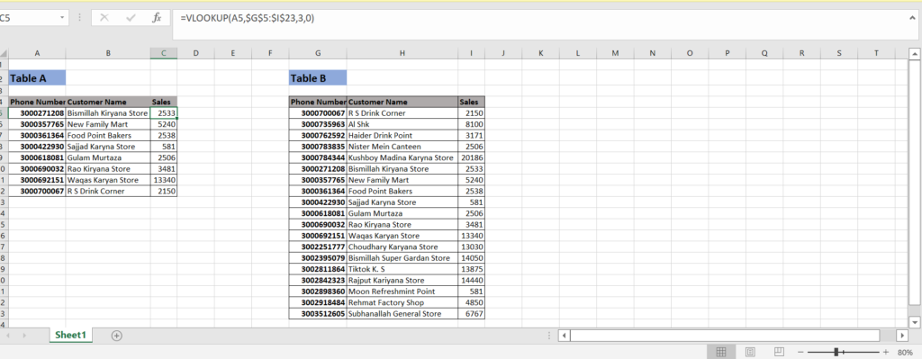
This way is most common when the data does not change often and there are a few columns or rows you want to reference. Please see the below vlookup formula. We show a sample of how to use a vlookup formula in Microsoft Excel.

=VLOOKUP(A12,$G$5:$I$23,3,0)

Enter the formula by typing =VLOOKUP () in cell “A12”.
Type in the value (A12) you want to find
Step 3: Type in an equal sign and then type the column letter (In this case, we type “$G$5:$I$23” to refer to a range of column G to I in the same.
Type in the range of rows 3 to find matching data (In this case, we type “3” to refer 3 rows.
Type 0 after row number to get the value only instead of entire reference.
Press Enter to complete the formula.
Now, you can see that the vlookup formula has a function to search for specific data in one column or row and show data in another column or row.

how vlookup works in excel

First, create a table of data with a unique identifier in the leftmost column. For example, you might have a table of employees with employee IDs in the first column.
Next, select the cell where you want the VLOOKUP result to appear.
Click the “Formulas” tab in the ribbon at the top of the Excel window, then click the “Lookup & Reference” button in the ribbon.
Click “VLOOKUP” to bring up the function’s arguments.
In the “Lookup_value” field, enter the value that you want to search for in the table. For example, if you want to look up an employee’s name based on their ID, you would enter the ID in this field.
In the “Table_array” field, enter the range of cells that contains the table of data. For example, if your table is in cells A1 to D10, you would enter “A1:D10” in this field.
In the “Col index_num” field, enter the number of the column that contains the information you want to extract. For example, if you want to extract the employee’s name, which is in the second column of the table, you would enter “2” in this field.
In the “Range_lookup” field, enter either “TRUE” or “FALSE”. If you enter “TRUE”, Excel will find the closest match to the lookup value if an exact match is not found. If you enter “FALSE”, Excel will only return a result if an exact match is found.
Press “Enter” to complete the function. The VLOOKUP result will appear in the selected cell.

How to Use Vlookup in Google Sheets

VLOOKUP is a powerful function in Google Sheets that allows you to search a table of data and extract specific information from it. Here’s how you can use it:

First, create a table of data with a unique identifier in the leftmost column. For example, you might have a table of employees with employee IDs in the first column.
Next, select the cell where you want the VLOOKUP result to appear.
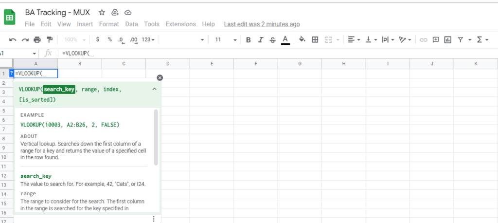
Type “=VLOOKUP(“ to start the function.
In the “search key” field, enter the value that you want to search for in the table. For example, if you want to look up an employee’s name based on their ID, you would enter the ID in this field.
In the “range” field, enter the range of cells that contains the table of data. For example, if your table is in cells A1 to D10, you would enter “A1:D10” in this field.
In the “index” field, enter the number of the column that contains the information you want to extract. For example, if you want to extract the employee’s name, which is in the second column of the table, you would enter “2” in this field.
In the “is sorted” field, enter either “TRUE” or “FALSE”. If you enter “TRUE”, Google Sheets will assume that the lookup column sorted the table and will use a faster search algorithm. If you enter “FALSE”, Google Sheets will search the entire table for the lookup value.
Close the function with a “)” and press “Enter” to complete it. The VLOOKUP result will appear in the selected cell.

Uses Of Vlookup Functions

The vlookup formula can be used to solve many different types of problems. The use of a vlookup formula allows you to find specific values in one column or row of data and shows all matching data in another column or row.

The vlookup formula can also be used in a table of data that does not have good header labels.

Looking up and retrieving data from a table based on a unique identifier such as an employee ID, product code, or account number.
Consolidating data from multiple tables or sheets into a single sheet or report.
Validating data by comparing it to a reference table.
Creating dynamic dashboards or reports that update automatically when the underlying data changes.
Combining data from different sources and performing calculations on it.
Cleaning and preparing data for analysis or machine learning.

VLOOKUP syntax

In Excel, the syntax for the VLOOKUP function is as follows:

VLOOKUP(lookup_value, table_array, col_index_num, [range_lookup])

In Google Sheets, the syntax for the VLOOKUP function is slightly different:

VLOOKUP(search_key, range, index, [is_sorted])

lookup_value (Excel) or search_key (Google Sheets): The value you want to search for in the table.
table array (Excel) or range (Google Sheets): The range of cells that contains the table of data.
col index_num (Excel) or index (Google Sheets): The number of the column that contains the information you want to extract.
range_lookup (Excel only): A logical value that specifies whether you want Excel to find an exact match or an approximate match for the lookup value. If you enter “TRUE” or leave this argument blank, Excel will find the closest match if an exact match is not found. If you enter “FALSE”, Excel will only return a result if an exact match is found.
is sorted (Google Sheets only): A logical value that specifies whether you want Google Sheets to assume that the table is sorted by the lookup column. If you enter “TRUE”, Google Sheets will use a faster search algorithm. If you enter “FALSE” or leave this argument blank, Google Sheets will search the entire table for the lookup value.

Learn More
What Is MS Excel Filter? How To Add Or Remove Filter In Excel, Uses And Shortcut Keys Of Filter

13 Best Advanced Features And Uses Of MS Excel

List Of Top 15 Advantages Of Ms Excel